![]()
Spectrum Recovery Competition, 2011
|
Spectrum Recovery Competition, 2011 |
|
The competition has concluded. Congratulations to Dr. Adrian Cable of Light Blue Optics, who is the winner with a final score of 597.
For those who are interested, the actual illuminant spectral power distributions are available as tab delimted text here. More detail on how the contest images were produced is available in this zip archive. See the ReadMe.txt file in the archive. That file is also available here.
PowerPoint slides of the presentation on the contest at the 2011 OSA Fall Vision Meeting.
We have provided a set of 10 test images. The contest is to estimate the relative illuminant spectrum for each of these images. The winning entry will be the one that has the minimum estimation error, averaged across the 10 images.
The winning entry will receive a prize of $1000, plus an invitation to present the method at the OSA Fall Vision Meeting, 2011.
Here is information on how to enter, as well as the rules for the contest.
Each image is a rendering of a scene. The spectral power distribution of the scene illuminant and of diffuse reflectance of each object in the scenes was specfied on a wavelength-by-wavelength basis, and the scene was rendered separately for each wavelength to produce a hyperspectral image. From the hyperspectral images, we computed the L, M, and S coordinates for the human cones at each image pixel.
Although the geometry of the lightsources in each scene may (or may not) be complex, each light source within a single scene had the same relative spectral power distribution.
Materials in the scene were specified within the isotropic Ward model [1]. Some scenes contained objects with only diffuse surface spectral reflectance. In other scenes, one or more of the objects contained a specular component. When present, the spectral reflectance of the specular component was spectally flat.
Scenes are rendered using the Radiance software package [2] via the RenderToolbox [3] wrappers. Radiance has many parameters. We note here only that the images were rendered using perspective projection and that the parameters were set to simulate the effect of mutual illumination between surfaces. Several published papers employ the general rendering methods used here [4].
We have provided one image set along with the corresponding illuminant spectral power distribution. This may be useful for calibrating illuminant estimation algorithms. The illuminant is provided in a .mat file. It contains two variables. The variable spd_illumSpdCal is a 31-dimensional column vector containing the illuminant spectrum. The vector S_illumsSpdCal is [400 10 31], which means that the spectral data in the three columns of B_illum are sampled at starting wavelenth 400 nm in 10 nm increments, with 31 wavelength samples (i.e. 400-700 nm in 10 nm increments).
All illuminant spectral power distributions, surface reflectance spectra, and cone fundamentals are sampled at 10 nm intervals between 400 and 700 nm inclusive.
All contest data files are provided as MATLAB [5] .mat files.
Illuminant Spectral Power Distributions
All illuminant spectral power distributions are constructed as a weighted sum of three basis functions, with the weights constrained that illuminants do not have negative power at any wavelengths. The three basis functions are provided in the file B_illum.mat. This file contains two variables, the 31 by 3 matrix B_illum and the 3 by 1 vector S_illum. The three columns of the variable B_illum are the spectral basis functions, in arbitrary energy units. The vector S_illum is [400 10 31], which means that the spectral data in the three columns of B_illum are sampled at starting wavelenth 400 nm in 10 nm increments, with 31 wavelength samples (i.e. 400-700 nm in 10 nm increments).
The diffuse component of all surface reflectance functions areconstructed as a weighted sum of three basis functions, with the weights constrained that surfaces do not have negative reflectance at any wavelengths. The three basis functions are provided in the file B_sur.mat. This file contains two variables, the 31 by 3 matrix B_sur and the 3 by 1 vector S_sur. The three columns of the variable B_sur are the spectral basis functions. The vector S_sur is [400 10 31], which means that the spectral data in the three columns of B_sur are sampled at starting wavelenth 400 nm in 10 nm increments, with 31 wavelength samples (i.e. 400-700 nm in 10 nm increments).
Cone coordinates are computed with respect to the Stockman-Sharpe 2-degree fundamentals [6]. These are in the file T_cones_osa.mat. This file contains two variables, the 3 by 31 matrix T_cones_osa and the 3 by 1 vector S_cones_osa. The three row of the variable T_cones_osa are the L, M, and S cone fundamentals, in arbitrary energy units. The vector S_cones_osa is [400 10 31], which means that the spectral data in the three columns of T_cones_osa are sampled at starting wavelenth 400 nm in 10 nm increments, with 31 wavelength samples (i.e. 400-700 nm in 10 nm increments).
For each image, the error measure will be computed as follows. Let eTrue be a 31 by 1 vector containing the relative illuminant spectral power distribution used to render the scene. Let eEst be a 31 by 1 estimate of this vector. We will find the scale factor k such the k*eEst minimizes the mean squared error over wavelength between eTrue and k*eEst. This minimized mean squared error is then taken as the error for the estimate eEst. The overall error score is the mean over images of this minmized mean squared error. See the sample program for code that computes the error.
This sample MATLAB program implements a simple gray world illuminant estimation algorithm [7], and illustrates how to read the data, how to store the estimates in a single matrix, and how the overall error score is computed. [Obviously, it won't compute the error for you because you don't know the actual scene illuminants. But, it shows how the computation goes.] The algorithm implemented in this program produces an error score of 3544.88. This score is posted on the leaderboard under the name grawWorld. The output of the sample program is also provided as the text file estimatedIllumSpds.txt.
Paul Ivanov has provided a Python version of the sample program. Thanks!
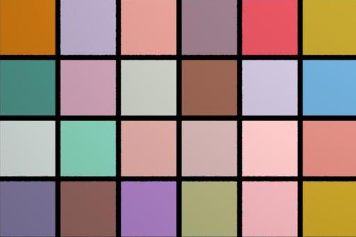
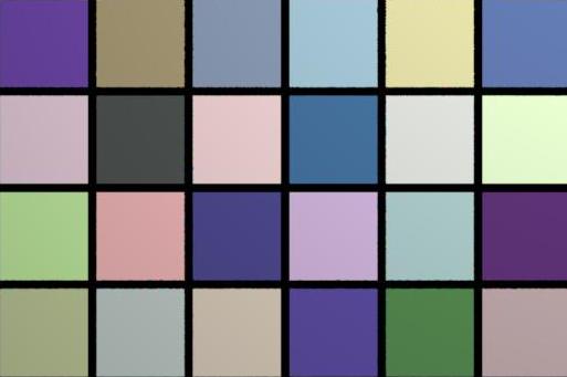
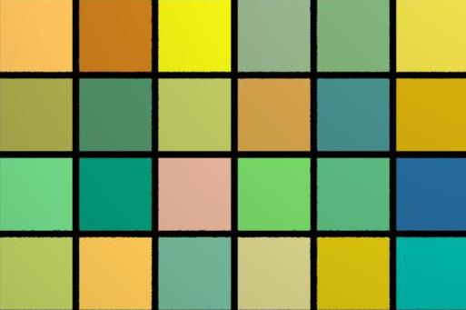
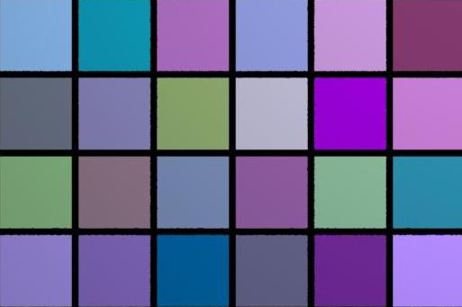
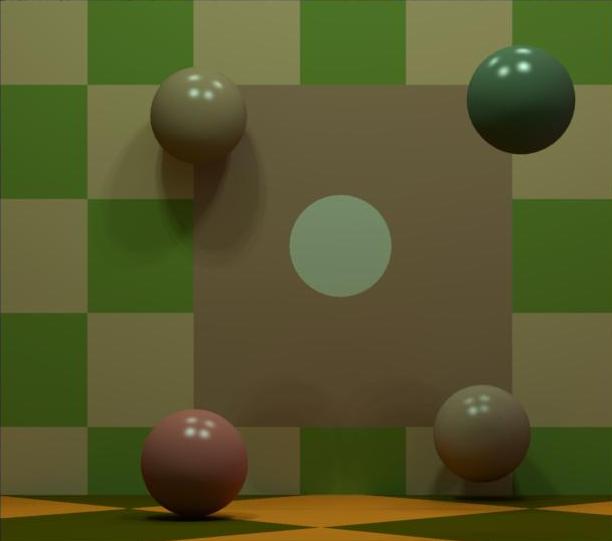
For each image, we provide the LMS cone coordinates in a MATLAB .mat file. Each of these images contains a N by M by 3 matrix called theImage. The L, M, and S planes provide the L, M, and S cone coordinates at each pixel respectively. We also provide an JPEG rendering of each image. These are simply for visualization and should not be used as actual image data for the contest - these images were scaled and/or tone-mapped by hand to produce reasonable looking images for display. The archive also contains the calibration image and its illuminant spectrum. For fun, the jpeg images are shown below.
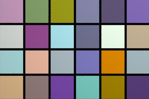
Calibration Image:
|
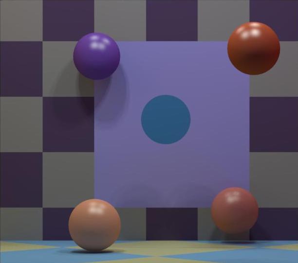
Image 1:
|
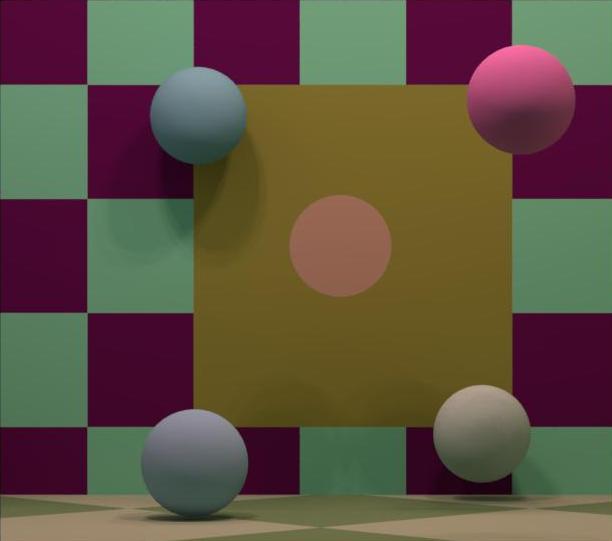
Image 2:
|
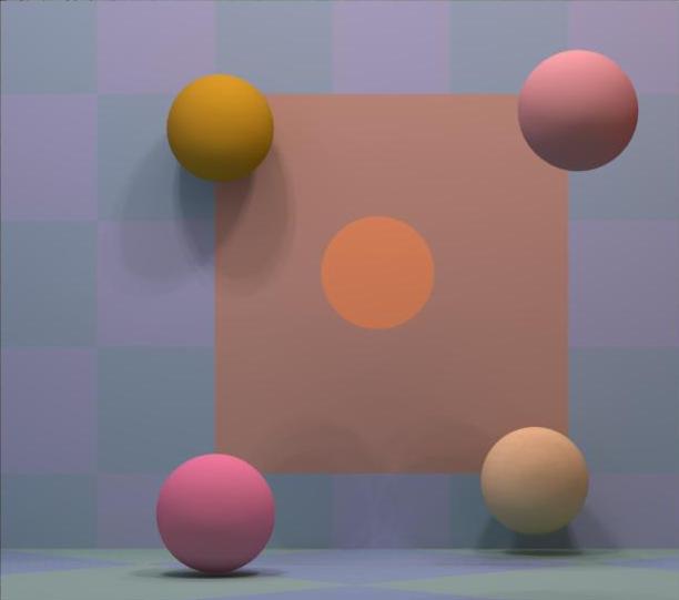
Image 3:
|
Image 4:
|
Image 5:
|
Image 6:
|
Image 7:
|
Image 8:
|
Image 9:
|
Image 10:
|
Posted here are any email exchanges in which we responded to questions about the challenge, and where we thought the information might be of use to others.
>From: David Brainard
>Date: February 16, 2011 9:50:32 PM EST
>To: Bill Freeman
>Subject: Re: spectrum estimation
>Hi Bill,
>All good questions. I think I should probably post this exchange on a FAQ, so that all contestants have access to the same information.
>Will do that momentarily.>>Some questions regarding the spectral challenge / upcoming problem set
>>for my class:>>I want them to do a straightforward illuminant estimation method, then
>>as extra credit / class project possibilities, let them explore
>>marginalizing over the surfaces.>>Do you have suggestions for good class assignment color constancy
>>algos? Grey world is great, but is already implemented for them.
>We review a number of algorithms in our 1997 JOSA paper (Brainard, D. H. and W. T. Freeman (1997).
>"Bayesian color constancy." Journal of the Optical Society of America A 14(7): 1393-1411) and
> provide references for them. So that's one source, although it won't contain post-1997 work.>A more recent source for ideas is Ebner, M. (2007). Color Constancy. Chichester, UK, Wiley.
>>I'll want them to make Gaussian models for the illuminant and
>>surfaces. Do you have suggestions for convenient ways for them to get
>>mean and variance values for those?>The Psychtoolbox distribution (http://psychtoolbox.org) contains spectral reflectance measurements for two sets of surfaces.
>These are in files sur_nickerson and sur_vrhel (in directory PsychColorimetricData/PsychColorimetricMatFiles). See the
>Contents.m file for description of data format. The sur_nickerson file is measurements of Munsell papers (Nickerson, D.
>and D. H. Wilson (1950). "Munsell reference colors now specified for nine illuminants." Illumination Engineering 45: 507-517.)
>The reference for the sur_vrhel file is Vrhel, M. J., R. Gershon, et al. (1994). "Measurement and analysis of object reflectance spectra."
>Color Research And Application 19(1): 4-9.>This web page has measurements of 2600 natural daylights: http://www.ugr.es/~colorimg/database.html
>>As a matter of principle, do you want only fully automated solutions?
>>ie, if a student wants to extract by eye the white patches of an
>>image, and use that in his calculation, is that ok?>There are no restrictions on how they get the estimates; algorithms, human augmented algorithms, human guesses, crowd-sourced solutions, etc. all OK.
>>They'll turn in their problem sets to us on March 2. Do you have any
>>preference on the timing of when they submit their solutions to you?>Anytime is fine. We are aiming for processing entries and returning scores about every two weeks, so there may be a lag before they find out how they did.
>Best,
>David
>>On Feb 19, 2011, at 9:21 PM, A. Kimball Romney wrote:
>>Dear Professor Brainard,
>>In the IMAGE DATA section on the second page of of the announcement of the OSA Spectrum Recovery Competition, 2011 it says,
>>"These are simply for visualization and should not be used as actual image data for the contest". Does that mean that an entry based on such use would be disqualified?
>>Thank you,
>>Kim Romney>Dear Kim,
>An entry can be made on any basis (algorithm, human guesses, crowd-sourced solutions, etc.), and can include the use of the rendered JPEG images as
>well as the supplied LMS cone coordinates. What was meant by the statement was simply that the rendered images are a depiction of the LMS data,
>and that the transformation between cone coordinates and the depicted images is not specified as part of the contest. Thus it might not be a good idea to
>use the depicted images, at least if your use relies on assumptions of how they were rendered. On the other hand, you are certainly welcome to use them.>Best,
>David
>P.S. I have started a FAQ on the contest page and am posting there any email responses I give to queries like this, so that all contestants have
> access to the same information. I will post this exchange there.
>From: David Brainard
>Date: March 1, 2011 8:21:13 AM EST
>To: Bill Freeman
>Subject: negative spectrum power
>Thanks.
>I took a slightly closer look, because if the rendering were perfect I don't think this would happen. That is,
>the specified scenes really do conform to the physical constraints specified on the web page.>I think what is going on is that for each spectral band, some combination of ray sampling and interpolation
>performed by Radiance produces a slightly different gradient across edges. This results in rendered
>spectra at some pixels that deviate from what a perfect renderer (i.e. the underlying physics) would
>produce and indeed values at some spectra that are not simple convex mixtures of values at neighboring
>pixels (which would also not lead to implied negative reflectance spectra.)>If you magnify the rendered images, you can see a slightly ragged look near some edges that is a symptom
>of this. If my assumption that the spatial structure of this raggedness differs across wavebands is correct (I
>did not check this explicitly), the effects described below are probably a second symptom.>Note also that simply filtering LMS = (0,0,0) doesn't detect all instances. Indeed, LMS = (0,0,0) pixels are OK
>because they will correspond to a reflectance of 0 at all wavelengths.>Best,
>David
>>David, A student in the class noted that some of the surface
>>coefficients in the calibration image of the contest web page, when
>>multiplied by the surface basis functions, give negative spectral
>>intensities. But as Michael (the TA) tracked down, these are all in
>>the black borders between color patches.>>--Bill
>From: David Brainard
>Date: March 20, 2011 11:22:34 AM EDT
>Cc: wade Wade
>Subject: Re: request for estimatedIllumSpds.txt>The output of the gray world sample program is now posted at:
>http://color.psych.upenn.edu/osacontest2011/estimatedIllumSpds.txt
>I have added this exchange to the FAQ. We would be happy to post your
>python program, or link to it if you put it up somewhere.
>Best,
>David
>>From: Paul Ivanov
>>Date: March 18, 2011 6:56:25 PM PDT
>>Subject: request for estimatedIllumSpds.txt
>>Hi David and Alex,
>>would it be possible for you to post estimatedIllumSpds.txt as
>>produced by the grayWorld example in SimpleIllumEstimation.m
>>I've reimplemented it using Python and want to verify that it is
>>running properly (both in terms of numerics and the desired
>>format).
>>I'll happily share the code once I know it is running properly.
>>(Also, it is not clear from the website if this is the
>>appropriate email address for questions, or if another email
>>address should be used)
>>best,
>>--
>>Paul Ivanov
[1] - Ward, G. J. (1992). Measuring and modeling anisotropic reflection. Paper presented at the SIGGRAPH '92: Proceedings of the 19th annual conference on computer graphics and interactive techniques.
[2] - http://radsite.lbl.gov/radiance/HOME.html ; see Larson, G. W., & Shakespeare, R. (1998). Rendering with Radiance: The Art and Science of Lighting Visualization. San Francisco: Morgan Kaufman Publishers.
[3] - http://rendertoolbox.org
[4] - Delahunt, P. B. and Brainard, D. H. (2004). Does human color constancy incorporate the statistical regularity of natural daylight? Journal of Vision, 4, 57-81 ; Xiao, B. & Brainard, D. H. (2008). Surface gloss and color perception of 3D objects. Visual Neuroscience, 25, 371-385 ; Olkkonen, M. & Brainard, D. H. (2010). Perceived glossiness and lightness under real-world illumination. Journal of Vision, 10(9:5).
[5] - http://mathworks.com
[6] - Stockman, A., & Sharpe, L. T. (2000). Spectral sensitivities of the middle- and long-wavelength sensitive cones derived from measurements in observers of known genotype. Vision Research, 40, 1711-1737.
[7] - Buchsbaum, G. (1980). A spatial processor model for object colour perception. Journal of the Franklin Institute 310: 1-26.