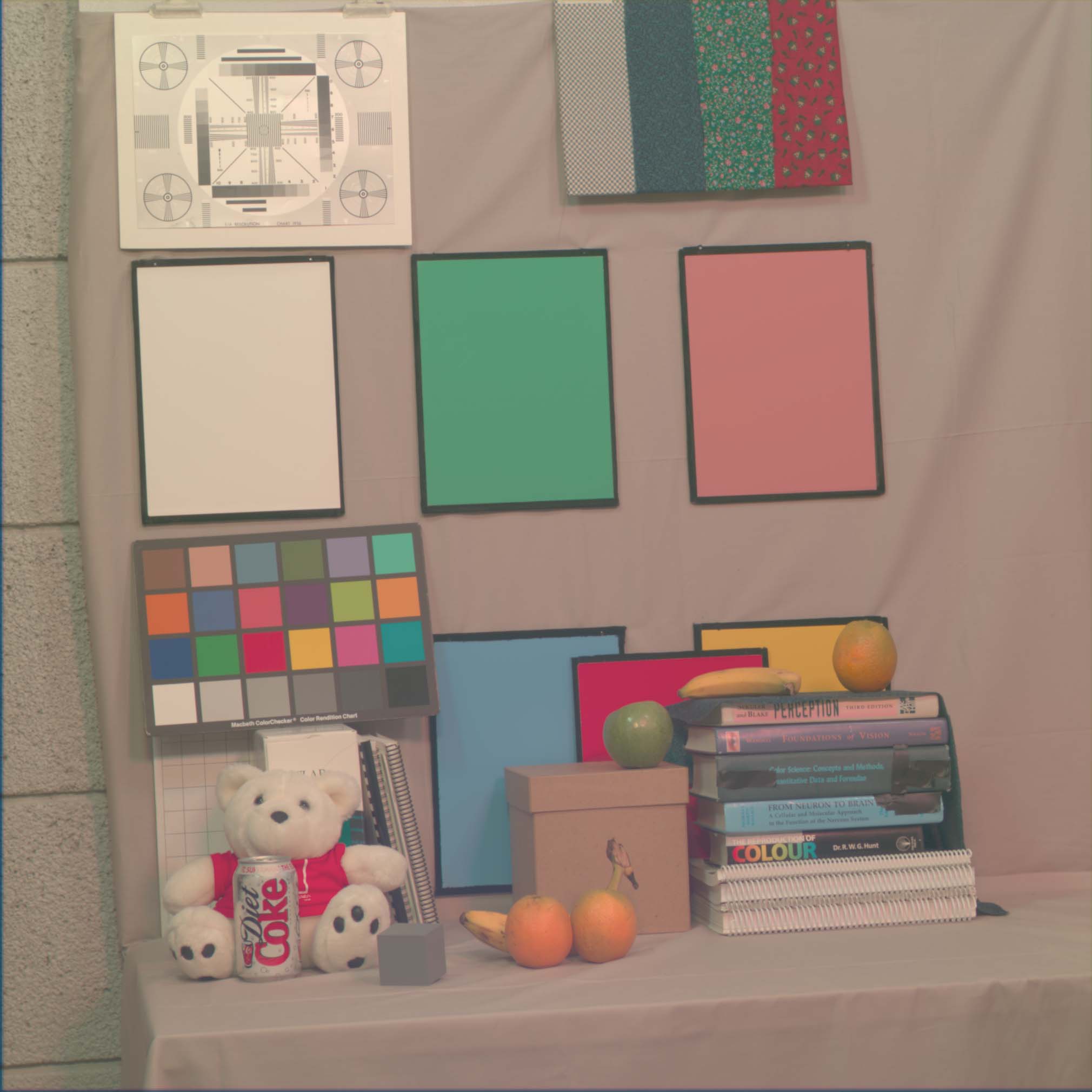
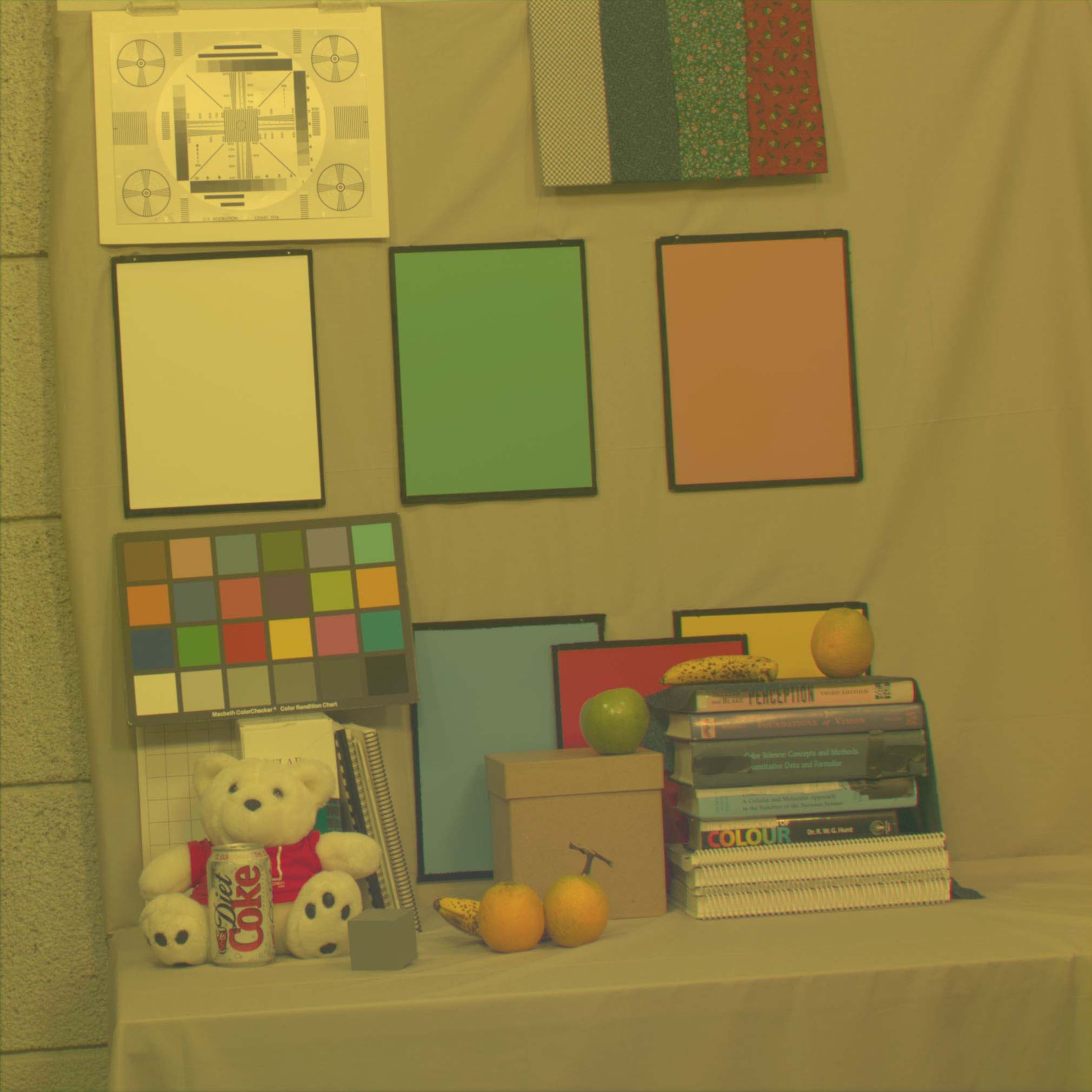
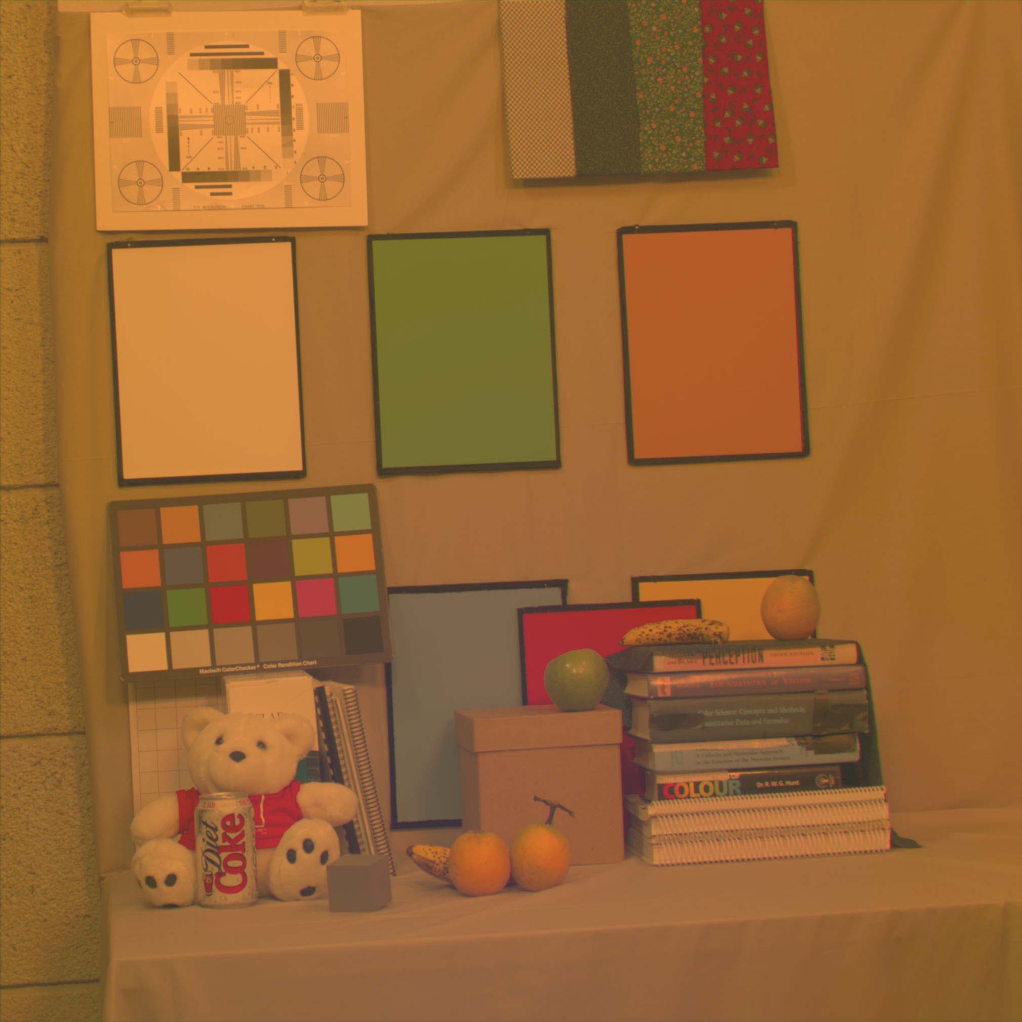
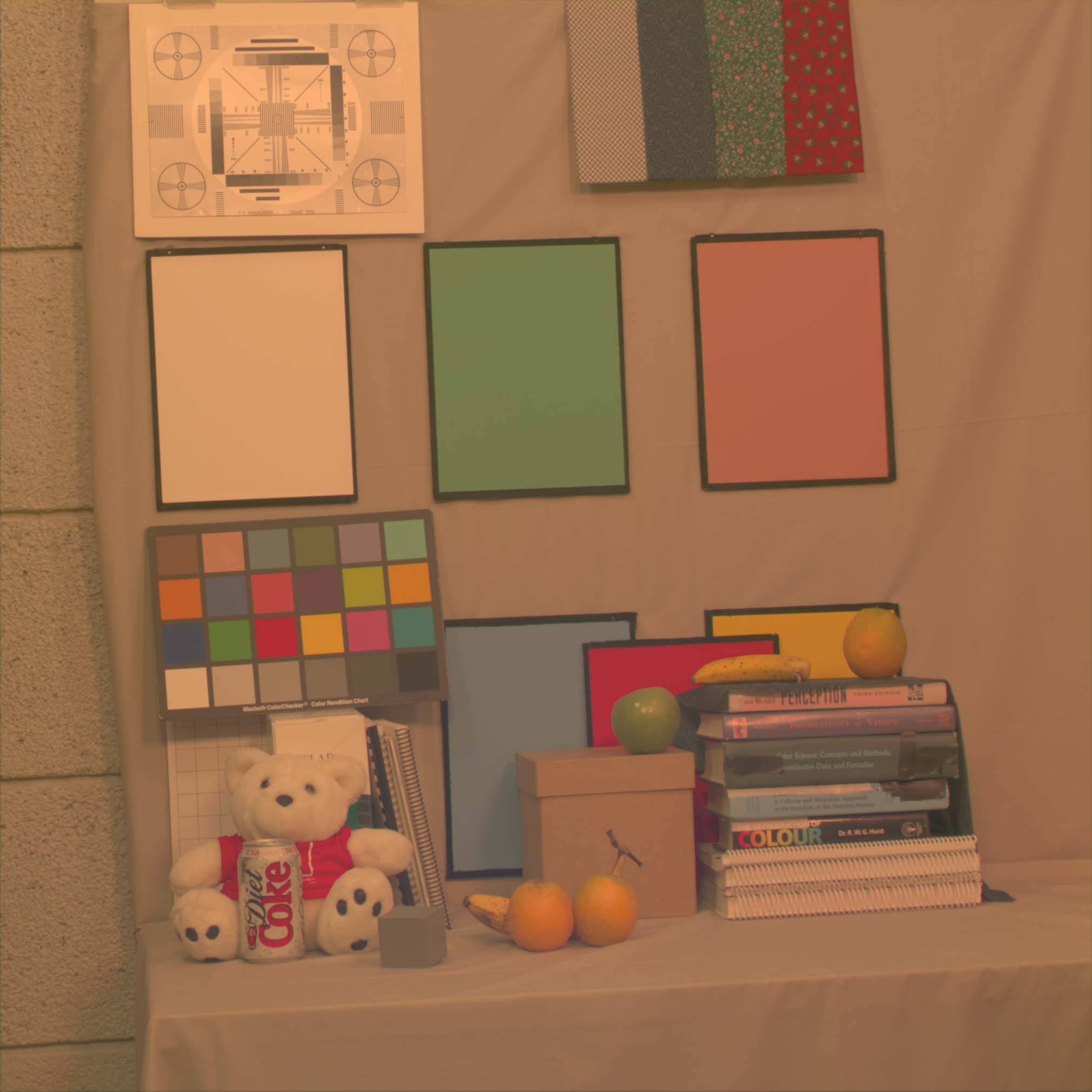
This page describes four hyperspectral images, which we refer to as the BearFruitGrayB, BearFruitGrayG, BearFruitGrayR and BearFruitGrayY images respectively. They were taken in a special laboratory room [5, 6] where the illumination was under computer control. The images are of the same set of surfaces under four different illuminants. The illuminants were bluish (B), greenish (G), redish (R), and yellowish (Y). You can view a plot of the four illuminant spectra (as measured reflected off of a matte Munsell N 9.5/ paper) by clicking here.
These images were acquired by E. A. Harding and myself as part of ongoing research on color image processing. You are welcome to use these images, but you should provide a citation [0], just as you would when you use data from any scientific publication. Other relevant references are provided here. (For example, Vora et. al [1] describe the initial camera design and a characterization of its performance for digital camera simulation.)
Each hyperspectral image consists of 31 monochromatic image planes, corresponding to wavelengths between 400 and 700 nm (inclusive) in 10 nm steps. The raw images are in provided in compressed UNIX tar format. For Macintosh users, this format is easily unpacked using the Stuffit application. The monochromatic images in the archive are named according to the convention 400, 410, .... 700. These individual images correspond to 400 nm, 410 nm, ..., 700 nm respectively.
Each monochromatic image is stored in a raw format as follows.
See image notes below for information on how to convert the raw data in the archives into radiometrically calibrated images.
For a listing of a MATLAB function that will read the individual images into a matrix variable, click here. (This function has only been tested on the Macintosh platform, last tested with version 2020a. On the way to the current version, Ted Cooper of Sony reported that there was a byte order problem under Windows. He supplied this MATLAB code fragment to fix that problem. Rajeev Ramanath of North Carolina State noted that in MATLAB R13 one can specify big or little-endian in the call to fopen, so that "fid=fopen('550_41', 'r', 'b'); data = fread(fid, [imSize,imSize], 'ushort'); fclose(fid)" should suffice to read the files, where imSize is the linear dimension of the image.)
To view a hyperspectral image, it is useful to reduce it to an RGB format. The RGB images are useful for obtaining a sense of the appearance of the image, but the values should not be used for calculations - they are specific to a particular monitor and rendering procedures. For calculations, the underlying spectral data should be used. For the images shown, the rendering to RGB was done in two basic steps. First, we used the hyperspectral images together with the CIE 1931 color matching functions to calculate the XYZ tristimulus values at each image location. We then used monitor calibration information (for an Apple 20" color monitor that was available in our lab) to compute RGB image values that produce an image that is pixel-by-pixel metameric to the XYZ image that was derived from the hyperspectral image. Some of the regions of the hyperspectral image were out of gamut -- producing the appropriate monitor metamer would require negative power on one or more guns, or more light than the monitor could produce. These were brought into gamut using some combination of scaling and clipping before gamma correction. The particular monitor data used for gamma correction has the feature that there is a relatively high-threshold before variation in input values has any effect on the light output. Because of this and the gamut mapping, the rendered images on this page can appear washed out. We have since developed procedures for producing nicer looking RGB images. Please contact David Brainard if you are interested knowing more about this particular issue.
From your browser you can view a full-sized JPEG version or download a full-sizedTIFF version. The JPEG versions load much more quickly but may have lost some fidelity due to the compresssion. If you are using an 8-bit (256 color) display, what you see is also subject to the dithering algorithm used by your browser. Also note that the gamma curve of your display can have a large effect on the appearance of the images. If you really care about how they look, you should rerender the images for your display.
1. The images were acquired by placing interference filters between the back of the lens and the CCD chip. This arrangement minimizes spatial artifacts in the images. But it has the effect of producing changes in image location and scale from filter to filter. (In addition, we have to refocus the camera for every filter.) To correct for this, we used a global affine motion estimation algorithm to compute transformations that register each image with the 550 nm image. We used code provided by Heeger that implements an algorithm described by Bergen et al. [8]. For more information on the registration software, go here.
The image registration software assumes that the only change from one image to the next is camera position. This is not the case for our images, as we also change wavelength. Images at different wavelengths exhibit the same basic spatial structure (as evaluated by eye), but the relative intensities between corresponding pairs of image regions are not preserved (that's what produces color). To handle this, we preprocessed the images with a simple edge extraction algorithm before registering them. We tried this in two ways. In one case, we preprocessed the entire image and passed the result to the multiscale alignment routine. In the other case, we ran the edge extraction algorithm separately on the representation at each scale in the registration process. In general, the two procedures produced similar results. As evaluated by eye, the first procedure produced better results (less chromatic fringing at edges), but it occaisionally failed to converge. We therefore checked the convergence and used the first procedure whenever it worked and the second procedure when the first failed.
Because of the registration proceedure, there is some distortion around the edges of the images. You should trim the edges off before performing any quantitative analyses.
2. For each image, we took a corresponding dark image and flat field image. The flat field image was acquired by aiming the camera into an integrating sphere. We dark corrected each image by subtracting the dark image. We also dark corrected the flat field image. We then corrected (to first order) for camera non-uniformities by dividing (pixel-by-pixel) each image by the corresponding (dark corrected) flat field image. To keep the scale of each image in the range of 16-bit integers, we multiplied the result of this procedure by the spatial mean of the flat field image.
After dark correction and flat fielding, we examined the responses from the 24 squares of the MacBeth Color Checker (MCC). Although we did not directly measure the spectrum coming from each of these squares, we have measured the reflectance function of each square (relative to the white square at the lower left of the chart). For each monochromatic image, then, we plot the measured response from each MCC square against the reflectance at the corresponding wavelength. The points in this plot should be well-fit by a line through the origin. We often found, however, that the best fitting line did not pass through the origin. This indicates the presence of stray light/signal that was not corrected for by our dark subtraction procedure. We believe that this light originates from small pinholes which are intrinsic to our interference filters. Although the stray light is probably not spatially uniform, we corrected as best we could by subtracting a constant value from the image so that the locus of measured response versus measured reflectance values passed through the origin. This correction was generally substantial only for shorter wavelengths.
3. The individual monochromatic images were taken using different f-stops and different exposure durations. To produce a calibrated hyperspectral image, each individual image must be scaled by a calibration factor. The calibration factors were determined by comparing the image data at a reference location to direct radiometric measurements (PhotoResearch PR-650) of the light coming from this location. After scaling, the image data provide power in units watts*m2*sr*10nm.
For the four images here, the reference location was the white paper in the left center of the images (location R in the locator image). The white paper was a Munsell matte N 9.5/ paper. To obtain an estimate of the illuminant incident at the reference location, multiply the reference spectrum by 1.12 at each wavelength. For each image, the calibration factors and reference spectrum are provided as a Macintosh text file, calibration.mtxt. The calibration file also contains the spectra measured at locations B, P, and G shown in the locator image. The calibration files are not included in the image archives but may be downloaded directly from your browser (see Image Data).
4. The four BearFruitGray images are not exactly registered with each other. They were taken on different days and the camera was repositioned between days. The objects in the scene were not moved, but there are some subtle differences in the object composition from image to image. In particular, the fruit was presumably a little riper when the BearFruitGrayG and BearFruitGrayR images were taken than it was for the BearFruitGrayB and BearFruitGrayY images. Also, a strip of masking tape was added to the light blue book in the scene for all but the BearFruitGrayB image. This was done to minimize glare.
5. For the BearFruitGrayB image, we have explicitly checked the camera spectral calibration by measuring reference spectra at three locations other than the white panel and comparing these spectra with the spectra derived from the hyperspectral image data. These comparisons can be viewed here.
6. We have not yet fully characterized the optical MTF of our camera system. Since we refocus for each individual wavelength, chromatic aberrations are probably minimized. The image of the resolution target could probably be used to estimate the spatial MTF at each wavelength.
7. The spatial resolution of the camera is 102.4 pixels per degree of visual angle.
8. If you would like to re-render the images yourself, the calibration data for our monitor is available in Macintosh text format. The file monspectra.mtxt contains the spectral power distributions of the monitor red, green, and blue phosphors. The units of power are watts*m2*sr*5nm, so that each value represents the power in a 5 nm band. The measurements are for the maximum output of each phosphor. The file mongamma.mtxt contains a table of the input-output relations for each monitor phosphor. Each table is normalized to one at its maximum value (input 255). This monitor has a extreme threshold for input before any light is output. You will probably obtain better rendering results if you simply gamma correct assuming a power function with an exponent of about 2. The file xyz1931.mtxt contains a tabulation of the CIE 1931 XYZ color matching functions. You could also render the images using the Smith-Pokorny estimates of the human cone spectral sensitivities, which are provided in the file conespectra.mtxt.
9. For many calculations you might want to perform on these images, it is useful to have linear models for the illuminant and surface spectra. The illuminants in our experimental room we produced by theater stage lamps passed through red, green, and blue dichroic filters. Although there are slight shifts in the spectra of the lights as we varied control voltage, a 3 dimensional linear model provides a good account of the illuminants we could produce. The file illummod.mtxt provides a 6 dimensional linear model for our room illuminants. The first 3 columns are the best available 3 dimensional linear model. (It is not the case, however, that the first 2 columns are the best 2 dimensional linear model. Use either 3 or 6 dimensions from this model.)
A useful linear model for surfaces may be derived from the reflectance spectra of the Munsell papers. A 6 dimensional version of such a linear model is provided in file surmod.mtxt. If you wish to use a smaller dimensional model, simply extract the first N (N <= 6) columns of the model.
10. We have estimated the noise properties of our images. For each of the four hyperspectral images, we replicated the 550 nm plane both at the start and finish of the image series. This gives us two replications (pre and post) of four image planes (550 nm plane for each hyperspectral image) for a total of eight independent image replications. We registered each of the pre and post images to its corresponding 550 nm image, then extracted a 30 by 30 pixel block of pixels from the center each square of the Macbeth Color Checker. To get a visual sense of the noise, we plotted the values from a replicated image against those for the original image. Such a plot is shown here for the BearFruitGrayB pre image. If there were no noise, then all the points would plot along the diagonal. Each cluster of points in the plot comes from one MCC square. (Note, the plot shows only a random subsample of the data that were analyzed quantitatively.) It is clear from the plot that the noise increases with the mean intensity level.
To get a more quantitative meausure of the noise, we proceeded as follows. We predicted each point in the pre/post image with the corresponding point from the main 550 nm image. For each MCC square, we then computed the variance of the residuals of these predictions, and also the mean level of response for all pixels from that square. A plot of the computed variance versus the mean level of response is shown here. If the noise were additive, the plot would be a horizontal line, which it clearly is not. If the noise were Poisson, the data would lie along a line through the origin with unit slope. This is also not an accurate model. We fit the data with an equation of the form V = k1 + k2*M^p, where V is the variance, M the mean, and k1, k2, and p are free parameters. This parametric form can describe additive (k2 = 0), Poisson (k1 = 0, k2 = 1, p = 1), and multiplicative (k1 = 0, p = 2) noise. The plot shows the fit for the data shown. The fit is quite good.
We repeated this process for all eight image replications and averaged the parameter values for k1, k2, and p. The averaged values are 17.02 +/- 9.18, 4.07E-03 +/- 5.36E-03, and 1.76 +/- 0.27, where the precision given is the standard deviation of the eight individual estimates.
It seems reasonable to assume that the noise depends on the mean pixel response and not on the image wavelength, but we have not yet checked this assumption explicitly.
BearFruitGrayB
image
BearFruitGrayG
image
BearFruitGrayR
image
BearFruitGrayY
image
The full image archives are rather large. Some people have requested the image in more digestable chunks. I have broken each image into 16 blocks (505 by 505 pixels each) and put each block into a separate archive. The block index ij follows MATLAB convention, with i representing the block row and j representing the block column. The format of the raw images in each block is the same as in the large archive, with the block index postpended to the individual filenames.
Listing of MATLAB code to read raw image
format
Plots of illuminant spectra for the BearFruitGray
images
Spectral calibration check for BearFruitGrayB
Obtain
Heeger's registration code
References
J. E. Farrell, E. A. Harding, J. M. Kraft, M. D. Rutherford, J. D. Tietz, and P. L. Vora helped with camera design, camera calibration, and/or image acquisition. D. J. Heeger provided the image registration code. Ted Adelson and Ron Smith wondered why the apparent contrast of some of the early images was low. This led to the improved dark correction procedure adopted for these images. The work was supported primarily by a philanthropic gift from the Hewlett-Packard Corporation.